How can models predict groundwater contamination?
Maps and Models to Predict the Groundwater Quality on GAP
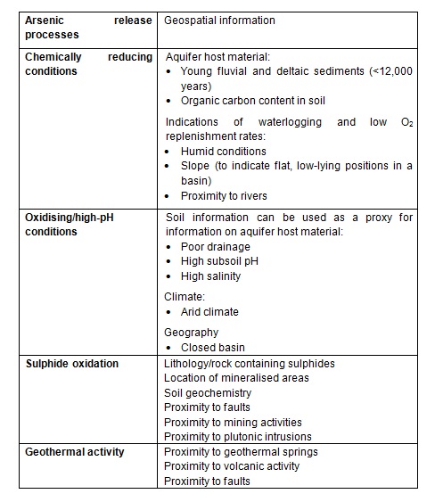
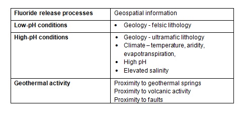
Continuous coverage of geospatial information is very useful for the development of predictive water quality models. The first step involves an initial selection of geospatial data that could be correlated to geogenic groundwater contamination (predictor or independent variables). This is a critical step that requires an understanding of the processes causing contaminant release, as described above. To aid in deciding which geospatial layers to use, a summary of release processes and typically associated data have been compiled for arsenic (Table A) and fluoride (Table B).

Table A - Arsenic release processes and examples of corresponding geospatial information (Terms of use: Cite original source from Handbook)

Table B - Fluoride release processes and corresponding geospatial information (Terms of use: Cite original source from Handbook)
The second step involves selecting the area for which a map is to be developed, which is divided into pixels (or squares). The pixel size depends on the resolution of the available data (1 km2 in GAP). The average value of the measured concentration data within each pixel is used for model calibration. For each measured data point (dependent variable), an iterative statistical analysis is made with the predictor variables to find the degree of positive or negative correlation between the two and to determine the coefficients of the model parameters. It is important to have a range of measured data values that encompasses a comparable proportion of high and low values. This spread of data is essential, since the model will be able to predict only across this same value range. In the case of logistic regression, where the dependent variable is taken to be either high or low (1 or 0), the cut-off between the two is commonly chosen to be the contaminant concentration limit determined by the authorities (e.g. WHO) as being acceptable for human consumption. The same is true for independent variables. For example, if the values of an independent variable are the same for all of the data points being modelled, this variable cannot explain any of the variance found in the data since the independent variable itself does not vary. It is therefore important in being able to establish a correlation that the dependent data points take in a broad range of independent variable values. This could then mean targeting a groundwater sampling campaign in specific regions with differences in, for example, geology or soil type and not necessarily where high arsenic levels are expected. A rule of thumb for the minimum size of the dataset (of the dependent variable) to be modelled is to have a ratio of at least 10 cases to every independent variable. In this instance, “cases” refers to the smaller of the number of high or low data values (1 or 0) in the dataset. For example, when using three independent variables with a dataset having 60% high values / 40% low values, the dataset should contain at least: 10 x 3 / 0.4 = 75 samples (REF).
It should be noted that in both low- and high-pH conditions there is a potential for elevated dissolved fluoride concentrations in groundwater because of limited dissolved calcium concentrations that could otherwise control dissolved fluoride concentrations by the precipitation of fluorite (CaF2(s)).
Below are some examples of our models for predicting groundwater quality in unmonitored areas
Global Maps of Groundwater Quality
Global threat of arsenic in groundwater
Statistical modeling of global geogenic arsenic contamination in groundwater
Statistical modeling of global geogenic fluoride contamination in groundwaters
National Maps of Groundwater Quality
Groundwater Arsenic Distribution in India by Machine Learning Geospatial Modeling
Prediction modeling and mapping of groundwater fluoride contamination throughout India
Local Maps of Groundwater Quality
The river-groundwater interface as a hotspot for arsenic release
Arsenic, manganese and aluminum contamination in groundwater resources of Western Amazonia (Peru)
Keywords
groundwater quality, geospatial data, geogenic groundwater contamination predictor, geospatial predictors, geospatial layers, contaminant release, processes, geospatial information, map, pixels, resolution, data, GAP, measured concentration, modelling, model, calibration, machine Learning, measured data point, statistical analysis, predictor, spatial, variables important, predict across, value range, logistic regression, local, global, statistical modeling, dependent variable, predicting groundwater quality, acceptable human consumption, independent variables, points, correlation, dependent data, groundwater sampling
For references, please visit the page
Health risks from the consumption of
How are health risks quantified?
Here you can find information about